
티스토리 뷰
@18.12.1
[PROLOG]
Image A
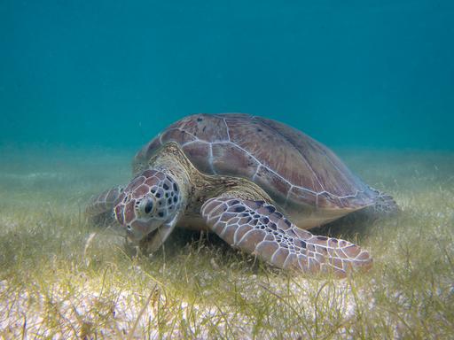
Image B
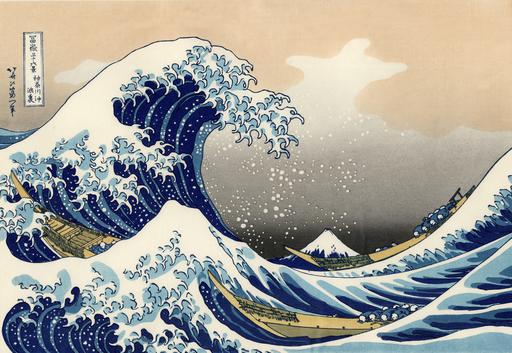
Image A+B
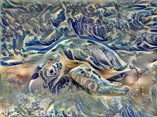
Image Style Transer 은 Image A와 Image B를 이용하여 새로운 그림을 만들어준다. 추 후 Style Transfer을 Sound에 적용하는 연구를 시도해보고자 Tensorflow Tutorial을 공부해보았다.
개념과 코드에 대한 설명이 섞여있기 때문에 코드만 또는 개념만 공부하고자 한다면 다소 복잡하고 지저분 할 수 있다. 코드와 개념을 같이 공부한다해도.. 많이 부족하여 지저분할 수 있다.
항상 개념만 공부하면 코드를 보았을 때 적용시키는 부분이 어려워, 코드와 개념을 함께 정리하여보았다.
1. 개요
Style Transfer의 원리는 2개의 함수로 정의된다.
: 두 이미지의 content가 어떻게 다른가
: 두 이미지의 style 차이
학습 대상의 (desired) content image, 학습 대상의 (desired) style image, 그리고 content image에 의해 초기화 될 input image 가 주어지게 된다.
input image 와 content image 의 를 minimize하고 input image 와 style image 의 을 minimize 하도록 학습하게된다.
Style Transfer에서는 빈 이미지 또는 무작위의 픽셀 값을 가진 이미지에서 시작한다. 학습을 통하여 바이어스, 가중치를 업데이트하고, Style Transfer에서는 바이어스, 가중치를 고정시키고 이미지를 생성한다.
2. Concepts
Tensorflow tutorial 에서는 최근 많이 활용되는 Eager Execution 을 활용한다. Eager Execution 은.. 정적인 flow 속에서 동작하였던 tensor flow 를 interpreter 와 같은 느낌의 대화형 프로그래밍이 가능하도록 해주는 것으로 최근 tensorflow tutorial 의 코드도 Eager Execution 을 활용하는 코드로 바뀌었다.
Functional API 를 사용하여 모델을 정의할 때 사용는 것 같은데.. 밑에서 살펴보자. 그리고 pre-trained model 을 사용하며, 위에서 정의한 Loss function 을 minimize 하기위하여 custom training loops를 사용한다.
3. Learning!
본 예제의 코드 구성은 다음과 같다.
Preprocessing input data
Define content and style Representations
Build Model
Define loss function
Apply style transfer to images
Computing the loss and gradients
3-1.Preprocessing input data
def load_img(path_to_img):
  max_dim = 512
  img = Image.open(path_to_img)
  print('[*]img.size : {}'.format(img.size))
  long = max(img.size)
  scale = max_dim/long
  img = img.resize((round(img.size[0]*scale), round(img.size[1]*scale)), Image.ANTIALIAS)
  print('[*]img.size after resize : {}'.format(img.size))
  img = kp_image.img_to_array(img)
  # We need to broadcast the image array such that it has a batch dimension
  img = np.expand_dims(img, axis=0)
  return img
먼저 load_img 함수 내에서는 이미지를 불러온 후 resize를 수행한다.
max_dim=512로 고정시켜놓고, 같은 비율이 되도록 세로 길이를 scale 한다.
위에서 밑으로 또는 밑에서 위 방향으로 행 단위로 입력되는 것을 알 수 있다.
def load_and_process_img(path_to_img):
  img = load_img(path_to_img)
  img = tf.keras.applications.vgg19.preprocess_input(img)
  return img
이 후 load_and_process_img 함수 내에서 tf.keras.applications.vgg19 모델의 전처리 과정을 수행한다.
vgg19.preprocess_input 에서는 image_utils.py 에서 정의된 함수를 이용하는데, 모델과 모드(tf, torch, caffe 등)에 최적화 되어있는 입력값의 평균, 편차 등이 정의되어있다.
본 예제는 vgg19 모델을 사용하기 때문에,
RGB -> BGR
mean = [103.939, 116.779, 123.68]
std = None
에 따라 input 값의 영역을 바꿔준다.
def deprocess_img(processed_img):
x = processed_img.copy()
if len(x.shape) == 4:
x = np.squeeze(x, 0)
assert len(x.shape) == 3, ("Input to deprocess image must be an image of "
"dimension [1, height, width, channel] or [height, width, channel]")
if len(x.shape) != 3:
raise ValueError("Invalid input to deprocessing image")
# perform the inverse of the preprocessiing step
x[:, :, 0] += 103.939
x[:, :, 1] += 116.779
x[:, :, 2] += 123.68
x = x[:, :, ::-1]
x = np.clip(x, 0, 255).astype('uint8')
return x결과 확인을 위하여 다시 역전처리 과정을 정의하였는데, 이 때에 값의 범위가 0~255를 벗어나는 픽셀에 대하여 np.clip 함수를 이용하여 min, max 값으로 대치한다.
3-2. Define content and style Representations
VGG19 모델을 사용할 때에, 최종 layer을 output이 아닌 intermediate layer의 output을 사용한다. style transfer에서 loss function define과 함께 왜 intermediate layer를 사용하는지가 중요한 것 같다. 이유는 Convolution Network와 같은 맥락이다. VGG19의 경우 이미지 분류 모델이며 이미지 분류의 경우 입력 이미지에 대한 기본적인 '이해'가 필요하고 이를 수행하는 것이 Convolution Network 이다.
Input image 마다 특성이 모두 다를지라도 Convolution Network 를 수행하며 공통적인 Feature를 찾게되고 같은 카테고리에 따라 유사한 Feature map이 많아지게 된다. Convolution layer 의 깊이에 따라 나타나는 특성이 모두 다른데, low layer부터 hight layer까지의 layer를 골고루 가져오므로써, 최대한 style image의 특성을 잘 유지하려는 것을 알 수 있다.
# Content layer where will pull our feature maps
content_layers = ['block5_conv2']
# Style layer we are interested in
style_layers = ['block1_conv1',
'block2_conv1',
'block3_conv1',
'block4_conv1',
'block5_conv1'
]
num_content_layers = len(content_layers)
num_style_layers = len(style_layers)위와 같이 VGG19 모델의 layer에 정의되어있는 각 layer의 이름을 통하여 intermediate layer를 사용한다. VGG19 모델은
block1_conv1 ~ block1_conv2
block2_conv1 ~ block2_conv2
block3_conv1 ~ block3_conv4
block4_conv1 ~ block4_conv4
block5_conv1 ~ block5_conv4
(activation = 'relu', padding = 'same')
로 구성되어 있는데 각 block의 conv5 layer 뒤에는 Maxpooling2D 연산이 수행된다.
Style layers에서는 각 block의 conv1만 사용하는 것을 볼 수 있는데, conv 연산 시 padding = same 에서 발생하는 loss를 고려해서 loss가 가장 적은 각 첫번째 conv layer를 사용한 것이 아닐까.. 예상해본다.
본 예제에서는 1개의 content_layers와 5개의 style_layers 를 정의하였다. input_image는 content_layer를 통하여 초기화되고 따라서 관련성이 깊기 때문에 적은 수의 레이어, style_layer는 보다 많은 layer를 사용하였다.
content_layers에 사용되는 'block5_conv2' 는 style_layers에 사용되는 layer들 직후에 존재하는 layer 이며 상위 layer에 속하는데, 이는 Style transfer에서 생성한 이미지가 입력 이미지와 가장 상위 layer에서 유사할 것이라는 직관에 근거한다. 이미지의 전체적인 느낌이 비슷하고, 이미지의 세부적인 느낌은 다르다고 생각하면 이해할 수 있다. content_layers에 사용되는 layer가 상위 layer일수록 전체적인 느낌(엣지, 형태 등)이 비슷해지고, 로우 레벨일수록 세부적인 느낌이 비슷해질 것이다. 따라서 content style을 결정할 때에는 중간, 하위 layer에서의 Loss가 크게 영향을 미치지 않는다고 볼 수 있기 때문에 상위 layer에 속한 output 한 층 만을 사용한다.
content_layers에는 5개의 layer가 사용된다. conv1~conv4까지 어느 layer를 사용할 지는 크게 중요하지 않은 것 같다. Style transfer의 성능을 개선하기 위한 몇몇 블로그들을 찾아보면, 개발자의 선택에 따라 각각 다른 conv layer를 사용하였음을 알 수 있다.
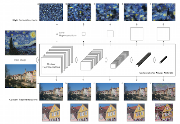
아래의 이미지를 보면 좀 더 이해가 쉽다!
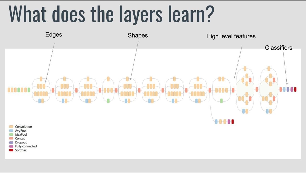
layer의 level에 따라 input image가 어떻게 변화하는지 확인해볼 수 있다.
3-3. Build Model
def get_model():
  """ Creates our model with access to intermediate layers.

  This function will load the VGG19 model and access the intermediate layers.
  These layers will then be used to create a new model that will take input image
  and return the outputs from these intermediate layers from the VGG model.

  Returns:
    returns a keras model that takes image inputs and outputs the style and
      content intermediate layers.
  """
  # Load our model. We load pretrained VGG, trained on imagenet data
  vgg = tf.keras.applications.vgg19.VGG19(include_top=False, weights='imagenet')
  vgg.trainable = False
  # Get output layers corresponding to style and content layers
  style_outputs = [vgg.get_layer(name).output for name in style_layers]
  content_outputs = [vgg.get_layer(name).output for name in content_layers]
  model_outputs = style_outputs + content_outputs
  # Build model
  return models.Model(vgg.input, model_outputs)
본 예제에서는 VGG19 모델을 사용하였다. Resnet, Inception 모델과 비교하였을 때 좀 더 단순한 구조로 인하여 Style 학습이 잘 이루어졌다고 설명되어있다.
style_outputs, content_outputs에서 위에서 정의했던 layer들을 가지고 온 다음에 (vgg.get_layer(name))
model_outputs = style_outputs + content_outputs
로 정의하였다. model_outputs은 GAN 모델과 같이 일반적인 이미지 출력이거나, Inception 등 Classifier 모델과 같이 어떠한 feature map이 아니라 style_outputs + content_outputs 로 이루어진 총 6개의 layer로 설정된다.
학습에 사용할 layers를 선택하여 이미지를 입력으로 받고 각 layer의 output을 출력으로 가지는 새로운 모델을 생성한다.
Functional API를 이용하여 간단하게 models.Model(vgg.input, model_outputs)로 구현하였다. Functional API는 keras에 정의되어있다.
3-4. Define loss function
a. Content Loss
는 간단하게 위와 같이 정의된다. 은 layer 을 뜻하며, 은 layer 에서의 Content Loss 를 뜻한다.
input image 에 대한 Convolution layer 에서의 출력인 와 content image 에 대한 Convolution layer 에서의 출력인 사이의 유클리디안 거리를 Content loss 로 정의한다.
and 이며, 는 layer 에서의 각 커널을 의미한다.
def get_content_loss(base_content, target):
  return tf.reduce_mean(tf.square(base_content - target))
b. Style Loss
Style Loss 는 총 5개의 layer로 구성되어 있었다. Style transfer에서 style이라는 것을 각 filter들 끼리의 correlation으로 정의한다. 이 때에 feature들 간의 correlation을 계산하기 위하여 Gram matrix가 사용된다. input_image, style_image의 feature 모두 Gram matrix로 변환된다.

이제 각 layer에서의 loss를 어떻게 정의하는 이 어떻게 구성되어있는지 알아보자.
은 layer 에서의 feature maps 의 수, 은 각 feature maps 의 를 뜻한다. Style Loss 또한 Content Loss 와 마찬가지로 유클리디안 거리를 계산하고 optimize를 수행한다. Style loss 를 계산할 때에 각 layer의 loss 를 그대로 모두 합하는 것이 아니라 각 layer의 loss별로 (가중치)를 두어 합한다.
위의 식은 로 해석된다. 과 같다. 은 전부 더하면 1이 되며, 으로 정의된다.
Content_loss, Style_loss를 각각의 특정 계수와 더하여 총 loss 를 구한다. 이 계수는 content와 style 어느쪽에 초점을 둘 지를 결정한다.

각 layer에서 filter들 사이의 correlation을 계산하기 위하여 Gram Matrix가 사용되며,
layer들 마다 고유의 filter 크기, filter 수를 가지는 것에 따른 영향을 줄이기 위하여 , 을 이용하여 값의 편차를 줄여 layer의 loss 를 계산한 다음에
layer loss마다 를 부여하여 Style loss 를 정의한다.
각 계수별로 곱한다음 서로 더하여 loss를 구한다.
여기에 대한 자세한 설명은 sanghyukchun님의 블로그를 참고하자.
def gram_matrix(input_tensor):
# We make the image channels first
channels = int(input_tensor.shape[-1])
a = tf.reshape(input_tensor, [-1, channels])
n = tf.shape(a)[0]
gram = tf.matmul(a, a, transpose_a=True)
return gram / tf.cast(n, tf.float32)
def get_style_loss(base_style, gram_target):
"""Expects two images of dimension h, w, c"""
# height, width, num filters of each layer
# We scale the loss at a given layer by the size of the feature map and the number of filters
height, width, channels = base_style.get_shape().as_list()
gram_style = gram_matrix(base_style)
return tf.reduce_mean(tf.square(gram_style - gram_target))# / (4. * (channels ** 2) * (width * height) ** 2)
get_style_loss 함수를 보면 get_content_loss 함수와 마찬가지로 tf_reduct_mean 을 사용하였음을 알 수 있다.
3-5. Apply style transfer to images
a. Optimizing
optimizing 기법으로는 Gradient descent , optimize function 으로는 Adam optimizer을 사용한다. 일반적인 optimizing에 있어 (가중치)를 업데이트하여 loss를 minimize 하는데, 본 tutorial 에서는 input image 를 update 한다고 설명되어있으며, 본 tutorial의 주된 목적과 벗어나기 때문에 L-BFGS를 사용하지 않았다고 되어있다.
* Note that L-BFGS, which if you are familiar with this algorithm is recommended, isn’t used in this tutorial because a primary motivation behind this tutorial was to illustrate best practices with eager execution, and, by using Adam, we can demonstrate the autograd/gradient tape functionality with custom training loops.참고로 L-BFGS 는 2차 미분에 활용되는 Hessian matrix 를 계산할 경우 계산 및 유지비용을 완화시키는 하나의 알고리즘이다.
어떠한 objective function의 함수값을 최적화하는 optimization 문제에서 가장 기본적인 수학적 원리는 일차미분(기울기)와 이차미분(곡률)의 개념이다. 이차미분을 활용할 경우
변곡점에서 불안정한 특성을 보인다.
이동할 방향을 결정할 때 극대, 극소를 구분하지 않는다.
는 문제점이 발생한다. 이를 해결하기위한 여러 방법 중 Quasi-Newton 이라는 방법이 있고 이 중 대표적으로 사용되는 방법이 BFGS 에 기반한 L-BFGS 이다.
이에 대한 설명은 개인적으로 정말 좋은 블로그라 생각되는 darkpgmr 님의 글을 참고하자.
b. get_feature_representations
아래 코드에서 Content Image 와 Style Image 가 pre-processing 되어 training에 사용되기 까지의 변화를 살펴보자.
Style transfer 의 custom model에는 vgg19 의 layer에서 style_layers에 사용되는 layer 5개와 content_layers에 사용되는 layer 1개를 더하여 총 6개의 layer가 존재하기 때문에
content_outputs[:5] => style_layers
content_outputs[5] => content_layers
를 의미한다.
def get_feature_representations(model, content_path, style_path):
"""Helper function to compute our content and style feature representations.
This function will simply load and preprocess both the content and style
images from their path. Then it will feed them through the network to obtain
the outputs of the intermediate layers.
Arguments:
model: The model that we are using.
content_path: The path to the content image.
style_path: The path to the style image
Returns:
returns the style features and the content features.
"""
# Load our images in
content_image = load_and_process_img(content_path)
style_image = load_and_process_img(style_path)
# batch compute content and style features
style_outputs = model(style_image)
content_outputs = model(content_image)
# Get the style and content feature representations from our model
style_features = [style_layer[0] for style_layer in style_outputs[:num_style_layers]]
content_features = [content_layer[0] for content_layer in content_outputs[num_style_layers:]]
return style_features, content_featuresload_img() 함수를 실행하면 다음과 같이 Image의 size가 변화된다.
[*]Content Image
img.size : (3367, 2525)
img.size after resize : (512, 384)
[*]Style Image
img.size : (4335, 2990)
img.size after resize : (512, 353)
Content Image 의 layer별 크기
#model(content_image)
[*]content_outputs :
[<tf.Tensor: id=188546, shape=(1, 384, 512, 64), dtype=float32, numpy=
array([...], dtype=float32)>,
<tf.Tensor: id=188557, shape=(1, 192, 256, 128), dtype=float32, numpy=
array([...], dtype=float32)>,
<tf.Tensor: id=188568, shape=(1, 96, 128, 256), dtype=float32, numpy=
array([...], dtype=float32)>,
<tf.Tensor: id=188589, shape=(1, 48, 64, 512), dtype=float32, numpy=
array([...], dtype=float32)>,
<tf.Tensor: id=188610, shape=(1, 24, 32, 512), dtype=float32, numpy=
array([...], dtype=float32)>,
<tf.Tensor: id=188615, shape=(1, 24, 32, 512), dtype=float32, numpy=
array([...], dtype=float32)>]
#[content_layer[0] for content_layer in content_outputs[num_style_layers:]]
[*]content_features :
[<tf.Tensor: id=188651, shape=(24, 32, 512), dtype=float32, numpy=
array([...], dtype=float32)>]
Style Image 의 layer별 크기
#model(style_image)
[*]style_outputs :
[<tf.Tensor: id=188471, shape=(1, 353, 512, 64), dtype=float32, numpy=
array([...], dtype=float32)>,
<tf.Tenor: id=188482, shape=(1, 176, 256, 128), dtype=float32, numpy=
array([...], dtype=float32)>,
<tf.Tensor: id=188493, shape=(1, 88, 128, 256), dtype=float32, numpy=
array([...], dtype=float32)>,
<tf.Tensor: id=188514, shape=(1, 44, 64, 512), dtype=float32, numpy=
array([...], dtype=float32)>,
<tf.Tensor: id=188535, shape=(1, 22, 32, 512), dtype=float32, numpy=
array([...], dtype=float32)>,
<tf.Tensor: id=188540, shape=(1, 22, 32, 512), dtype=float32, numpy=
array([...], dtype=float32)>]
#[style_layer[0] for style_layer in style_outputs[:num_style_layers]]
[*]style_features :
[<tf.Tensor: id=188631, shape=(353, 512, 64), dtype=float32, numpy=
array([...], dtype=float32)>,
<tf.Tensor: id=188635, shape=(176, 256, 128), dtype=float32, numpy=
array([...], dtype=float32)>,
<tf.Tensor: id=188639, shape=(88, 128, 256), dtype=float32, numpy=
array([...], dtype=float32)>,
<tf.Tensor: id=188643, shape=(44, 64, 512), dtype=float32, numpy=
array([...], dtype=float32)>,
<tf.Tensor: id=188647, shape=(22, 32, 512), dtype=float32, numpy=
array([...], dtype=float32)>]
content_outputs, style_outputs를 보면 [0:5]까지는 block1~block5 끝단에서 수행되는 layers.MaxPooling2D 함수에 의해 shape[0], shape[1]이 반으로 줄어드는 것을 알 수 있다. shape[2] 는 각 layer 별 kernel의 수를 의미 한다.
outputs의 마지막 레이어에서는 shape[0], shape[1]이 변화하지 않는 것을 볼 수 있는데, 이는 outputs[4], output[5]가 서로 동일한 block5에 존재하기 때문에, pooling이 발생하지 않기 때문이다.
content_features, style_features 는 content_image, style_image에 따른 output에서 앞에서 설정한대로 각각 사용하게될 layer를 가져와 정의한다.
3-6. Computing the loss and gradients
a. Compute loss
코드가 길어서 일부만 넣을까하였으나.. 본 게시글에서 모두 확인하기 쉽도록 다 첨부하였다.
def compute_loss(model, loss_weights, init_image, gram_style_features, content_features):
"""This function will compute the loss total loss.
Arguments:
model: The model that will give us access to the intermediate layers
loss_weights: The weights of each contribution of each loss function.
(style weight, content weight, and total variation weight)
init_image: Our initial base image. This image is what we are updating with
our optimization process. We apply the gradients wrt the loss we are
calculating to this image.
gram_style_features: Precomputed gram matrices corresponding to the
defined style layers of interest.
content_features: Precomputed outputs from defined content layers of
interest.
Returns:
returns the total loss, style loss, content loss, and total variational loss
"""
style_weight, content_weight = loss_weights
# Feed our init image through our model. This will give us the content and
# style representations at our desired layers. Since we're using eager
# our model is callable just like any other function!
model_outputs = model(init_image)
style_output_features = model_outputs[:num_style_layers]
content_output_features = model_outputs[num_style_layers:]
style_score = 0
content_score = 0
# Accumulate style losses from all layers
# Here, we equally weight each contribution of each loss layer
weight_per_style_layer = 1.0 / float(num_style_layers)
for target_style, comb_style in zip(gram_style_features, style_output_features):
style_score += weight_per_style_layer * get_style_loss(comb_style[0], target_style)
# Accumulate content losses from all layers
weight_per_content_layer = 1.0 / float(num_content_layers)
for target_content, comb_content in zip(content_features, content_output_features):
content_score += weight_per_content_layer* get_content_loss(comb_content[0], target_content)
style_score *= style_weight
content_score *= content_weight
# Get total loss
loss = style_score + content_score
return loss, style_score, content_score먼저, style_weight와 content_weight가 loss_weights에 의해 초기화된다. (업데이트 되지 않는다.)
init_image를 통하여 model_outputs을 얻는다. (init_image는 업데이트된다.)
model_outputs 에서 style, content output features들을 얻은 다음에, 위에서 정의한 loss 를 계산한다.
style_weight, conent_weight를 곱하여 score를 구한다음 이를 더하여 loss를 계산한다.
위와 같은 과정으로 iteration 마다 loss를 계산하게 되는데, 이 함수는 아래의 compute_grade 함수 내부에서 수행된다.
b. compute_grads
def compute_grads(cfg):
  with tf.GradientTape() as tape:
    all_loss = compute_loss(**cfg)
  # Compute gradients wrt input image
  total_loss = all_loss[0]
  return tape.gradient(total_loss, cfg['init_image']), all_loss
iteration 마다 compute_grads가 실행되고, 이후 tf.GradientTape().gradient를 실행한다.
tf.GradientTape().gradient(target, source) 함수는 source 값을 target 함수의 미분식에 대입하여 output을 반환한다. Model layer들의 가중치를 업데이트 하지않고, 입력 이미지만을 업데이트 하기위하여 all_loss와 함께 tf.GradientTape().gradient()의 결과를 반환한다. all_loss 의 값은 입력 이미지가 얼마나 잘 생성되었는지를 비교하는 데에만 사용되며, 학습에는 사용되지않는다.
c. Optimization loop
코드가 길어 해당 블럭 내에 주석으로 설명하였고, iterations의 for문만 아래 설명하였다.
import IPython.display
def run_style_transfer(content_path,
style_path,
num_iterations=10,
content_weight=1e3,
style_weight=1e-2):
# We don't need to (or want to) train any layers of our model, so we set their
# trainable to false.
'''
모델을 생성한 후 layer의 trainable속성을 False로 수정한다.
'''
model = get_model()
for layer in model.layers:
layer.trainable = False
# Get the style and content feature representations (from our specified intermediate layers)
'''
Model에서 각 feature에 해당하는 layer를 선택한 후, style_features에 한하여 gram_matrix로 변환한다.
'''
style_features, content_features = get_feature_representations(model, content_path, style_path)
gram_style_features = [gram_matrix(style_feature) for style_feature in style_features]
'''
이미지를 로드하고 init_image를 초기화한다.
optimizer function을 생성한다.
'''
# Set initial image
init_image = load_and_process_img(content_path)
init_image = tfe.Variable(init_image, dtype=tf.float32)
# Create our optimizer
opt = tf.train.AdamOptimizer(learning_rate=5, beta1=0.99, epsilon=1e-1)
# For displaying intermediate images
iter_count = 1
# Store our best result
best_loss, best_img = float('inf'), None
'''
필요한 속성들을 정의하는데, 여기서 init_image를 제외한 값들은 업데이트되지 않는다.
'''
# Create a nice config
loss_weights = (style_weight, content_weight)
cfg = {
'model': model,
'loss_weights': loss_weights,
'init_image': init_image,
'gram_style_features': gram_style_features,
'content_features': content_features
}
# For displaying
num_rows = 2
num_cols = 5
display_interval = num_iterations/(num_rows*num_cols)
start_time = time.time()
global_start = time.time()
norm_means = np.array([103.939, 116.779, 123.68])
min_vals = -norm_means
max_vals = 255 - norm_means imgs = []
for i in range(num_iterations):
grads, all_loss = compute_grads(cfg)
print('[*]grads length: {}'.format(grads.numpy().shape))
loss, style_score, content_score = all_loss
opt.apply_gradients([(grads, init_image)])
clipped = tf.clip_by_value(init_image, min_vals, max_vals)
init_image.assign(clipped)
end_time = time.time()
if loss < best_loss:
# Update best loss and best image from total loss.
best_loss = loss
best_img = deprocess_img(init_image.numpy())
'''
이하 생략
'''compute_grads(cfg)에서 반환하는 grads, all_loss를 살펴보자. 먼저 all_loss의 loss는 init_image가 얼마나 잘 생성되었는지 비교하는데에만 사용되고 style_score, content_score 은 이후의 print문 내에서만 사용된다.
init_image의 학습은 grads를 통하여만 이루어지는데 opt.apply_gradients 함수에서 실행된다. minimize 함수는 compute_gradients와 apply_gradients를 모두 호출하는 함수이다.
apply_gradients(grads_and_vars, global_step=None, name=None)
로 정의되며, paramter의 grads_and_vars는 comput_gradients의 output과 같다.
Style transfer 에서는 compute_gradients가 필요하지 않으므로(comput_grads 함수를 따로 정의하였기 때문에) apply_gradients 만 수행한다.
input_image의 pre-processing 단계를 다시보면 입력 값의 범위를 vgg19 모델에 맞게 평균, 편차를 수정하였다. 따라서 init_image를 deprecess하기전에 값의 범위를 pre-processing 단계의 범위와 맞춰준다. 이 때 tf.clip_by_value 함수가 사용된다.
[*]init_image
array([[[[ 2.58587513e+01, -1.49500113e+01, -1.18824852e+02],
         [ 1.82877903e+01, -2.35837574e+01, -1.28358398e+02],
         [ 2.79158611e+01, -1.08873749e+01, -1.18786530e+02],
         ...,
[*]after clip
array([[[[  30.611084  ,  -10.174826  , -113.982     ],
         [  13.464827  ,  -28.405594  , -128.43858   ],
         [  32.104626  ,   -6.389164  , -114.2312    ],
         ...,
마지막으로 deprocess_img(init_image.numpy()) 를 수행하면 업데이트된 init_image가 멋지게 보여진다!!
끝.
마치며..
Image가 아닌 다른 데이터에 content, style features를 분리하여 style transfer을 하려고하는데.. 잘 되었으면 좋겠다.
개인 공부를 위해 작성하였으며, 내용 상의 오류가 있다면 알려주시면 정말 감사드리겠습니다.
[참고]
Leon A. Gatys' paper, A Neural Algorithm of Artistic Style
Understand reducing loss with gradient descent
- Total
- Today
- Yesterday
- Rolling
- butterworth
- TensorFlow
- numpy
- deep learning
- 터널링
- IRR
- PYTHON
- AWS
- pandas
- Computer science
- VPN
- Machine Learning
- tacotron
- style transfer
- signal
- FFT
- detrend
- database
- filter
- scipy
| 일 | 월 | 화 | 수 | 목 | 금 | 토 |
|---|---|---|---|---|---|---|
| 1 | 2 | 3 | 4 | 5 | ||
| 6 | 7 | 8 | 9 | 10 | 11 | 12 |
| 13 | 14 | 15 | 16 | 17 | 18 | 19 |
| 20 | 21 | 22 | 23 | 24 | 25 | 26 |
| 27 | 28 | 29 | 30 |